

 Jari Sochorová
 Weather forecasts several days ahead rely heavily on numerical weather prediction (NWP) models. Among the best known are IFS from the European Centre for Medium-Range Weather Forecasts (ECMWF), GFS from the US National Oceanic and Atmospheric Administration (NOAA), ACCESS from the Australian Bureau of Meteorology (BoM), and MSM from the Japan Meteorological Agency (JMA).
These are physics-based numerical models of the atmosphere that calculate its future state using physical laws and numerical methods.
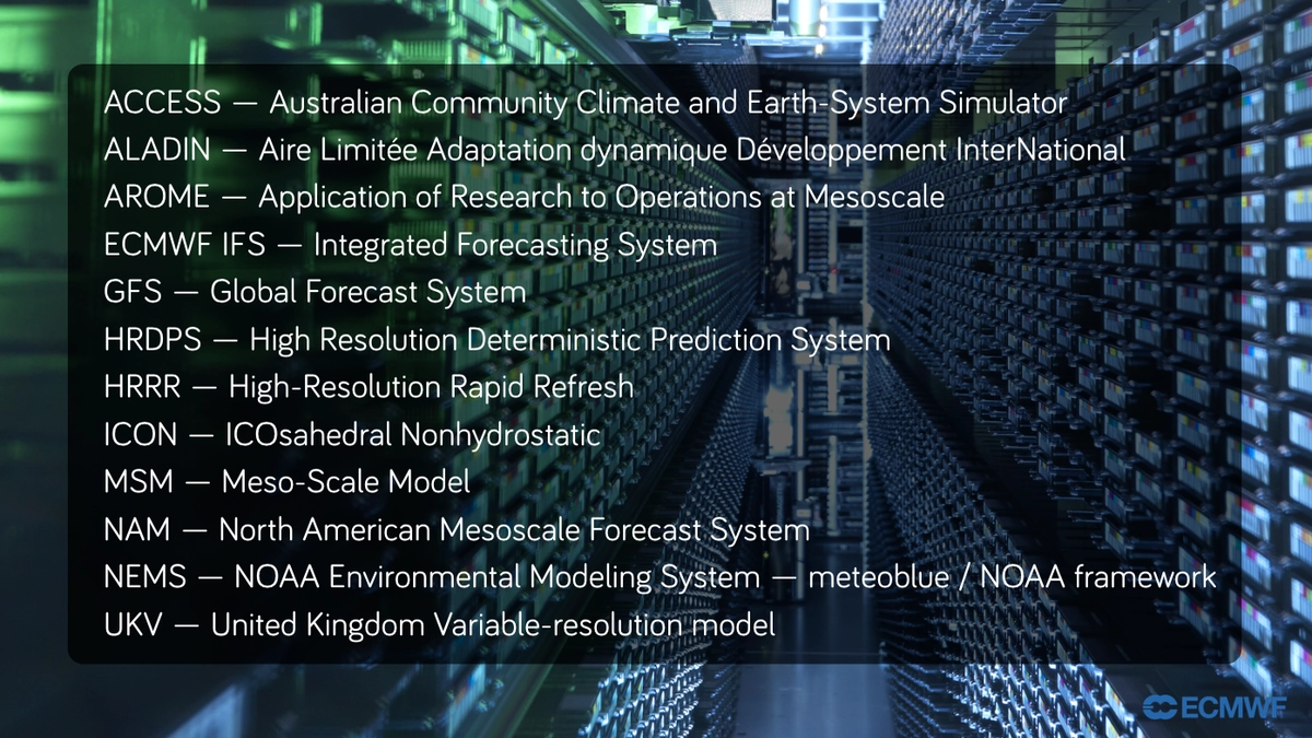
Meaning of the abbreviated names of some numerical models
In recent years, models based on artificial intelligence methods have also been developing rapidly. Initially, they were used mainly to improve the outputs of physics-based models, but today some can directly predict the future state of the atmosphere without the traditional numerical integration of physical equations. However, they still remain largely dependent on conventional NWP systems.
In the following text, we will take a simplified look at how traditional numerical weather prediction models are designed and how they produce a forecast.
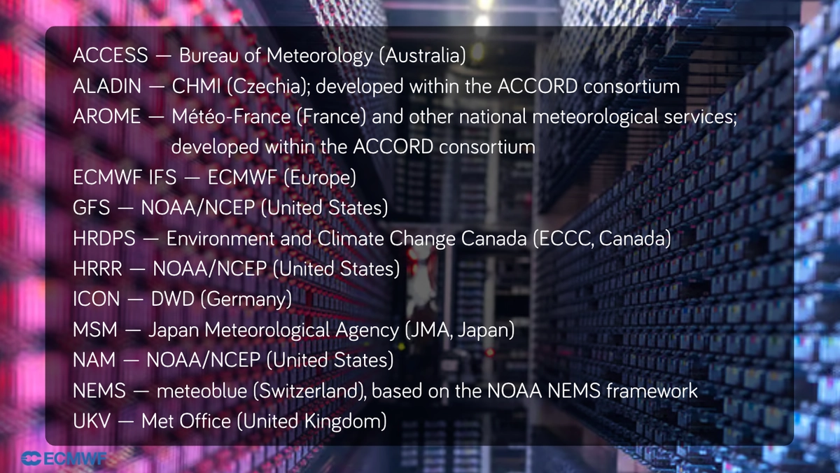
Models available on Windy.com and the centres that operate the configurations shown
The idea of forecasting weather using physical laws
The idea that the behaviour of the atmosphere could be described using physical laws was already being explored in the mid-19th century by Hermann von Helmholtz.
Around the turn of the 20th century, this gradually evolved into the idea that the future state of the atmosphere could actually be calculated. A major step was taken by the Norwegian physicist and meteorologist Vilhelm Bjerknes, who in 1904 formulated two basic requirements for such a forecast: we need to know the initial state of the atmosphere as accurately as possible and the laws governing its evolution.

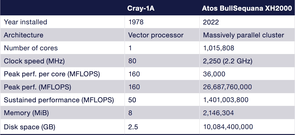
Two of the four clusters in ECMWF’s current Atos BullSequana XH2000 supercomputer system in Bologna, Italy, used to run operational weather forecasts and other high-performance computing tasks; ECMWF
Although meteorological observations, numerical methods and computing technology have changed beyond recognition since Bjerknes’s time, these two requirements remain at the heart of physics-based numerical weather prediction today.
From equations on paper to computer-generated forecasts
The British mathematician and physicist Lewis Fry Richardson was the first person to attempt a numerical weather forecast. He manually calculated the six-hour change in surface pressure at a single point for 20 May 1910. The calculation took him about six weeks and produced an unrealistic pressure change of 145 mb. He described his method in his 1922 book Weather Prediction by Numerical Process.
Although Richardson’s forecast was unsuccessful, his work laid the foundations for modern numerical weather prediction.
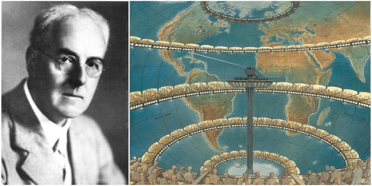
British mathematician and physicist L. F. Richardson envisioned a forecasting theatre with up to 64,000 “human computers” long before electronic computers existed, illustrated here by François Schuiten; Met Office; University College Dublin
A major breakthrough came with the development of electronic computers after the Second World War. In 1950, the first successful, though very simple, numerical weather forecast was produced using the ENIAC computer. The experiment was carried out by a team led by meteorologist Jule Charney, with mathematician John von Neumann also playing a major role.
At the time, calculating a 24-hour forecast took almost 24 hours. Nevertheless, the experiment demonstrated that numerical prediction of the atmosphere was feasible.
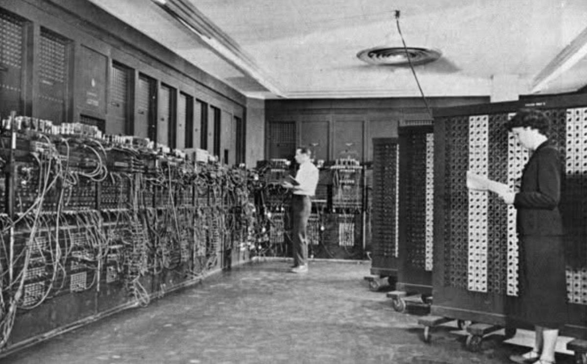
The ENIAC computer, which was also used to calculate some of the first numerical weather forecasts; U.S. Army via Wikipedia
Model dynamics: the equations governing the evolution of the atmosphere
We can think of the atmosphere as a layer of fluid moving over a rotating Earth. Its evolution is therefore governed by the physical laws describing fluid motion, while also accounting for the Earth’s rotation, gravity, and changes in pressure, temperature, and moisture.
At the core of a physics-based NWP model is a system of equations describing the dynamics and thermodynamics of the atmosphere. These include, in particular, the equations of motion, the continuity equation expressing conservation of mass, equations describing atmospheric moisture, the thermodynamic equation describing changes in energy, and the ideal gas law.
Together, these equations allow the model to calculate the evolution of so-called prognostic variables, typically including the wind components, temperature and moisture. Depending on the specific model, other prognostic variables may include pressure or density.
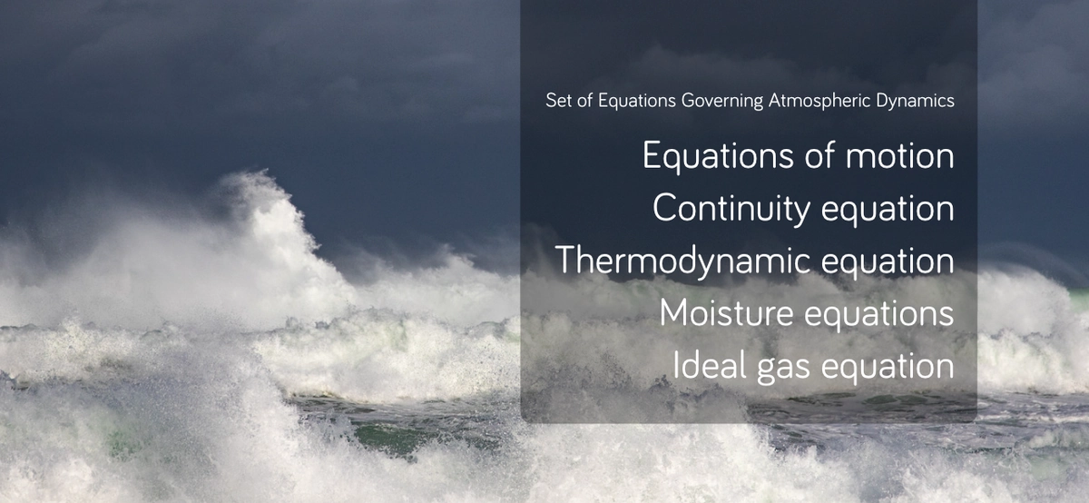
The fundamental equations themselves are largely similar across different models. The main differences lie in how they are solved numerically, what approximations (simplifications of reality) the model uses, and how it is designed within the limits of available computing power.
The equations describing atmospheric dynamics, together with the numerical methods used to solve them, form the model’s dynamical core.
Numerical methods: how to represent the atmosphere in a computer
The real atmosphere is continuous. Meteorological variables change smoothly in both space and time, but a computer can work only with a finite number of values. Space and time therefore need to be converted into a discrete form.
In the horizontal, the model divides the atmosphere into a computational grid, while in the vertical it uses a series of levels. At the points or within the cells of this three-dimensional grid, it works with discrete values of prognostic variables. The evolution of the atmosphere is also calculated in successive time steps.
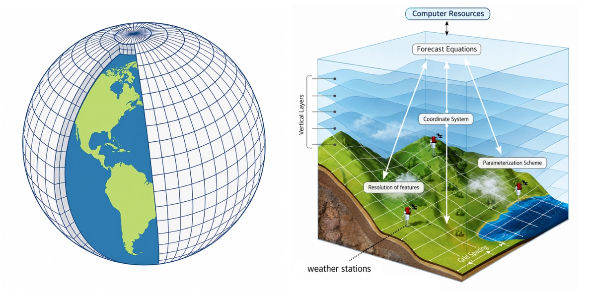
Illustrative model grid; meteoblue
Different numerical methods are used to obtain approximate solutions to the equations. Basic approaches include the finite-difference method, which replaces derivatives with approximate differences between values at neighbouring points; the finite-volume method, which tracks changes within individual grid cells; and spectral methods, which represent atmospheric fields as combinations of waves of different wavelengths.
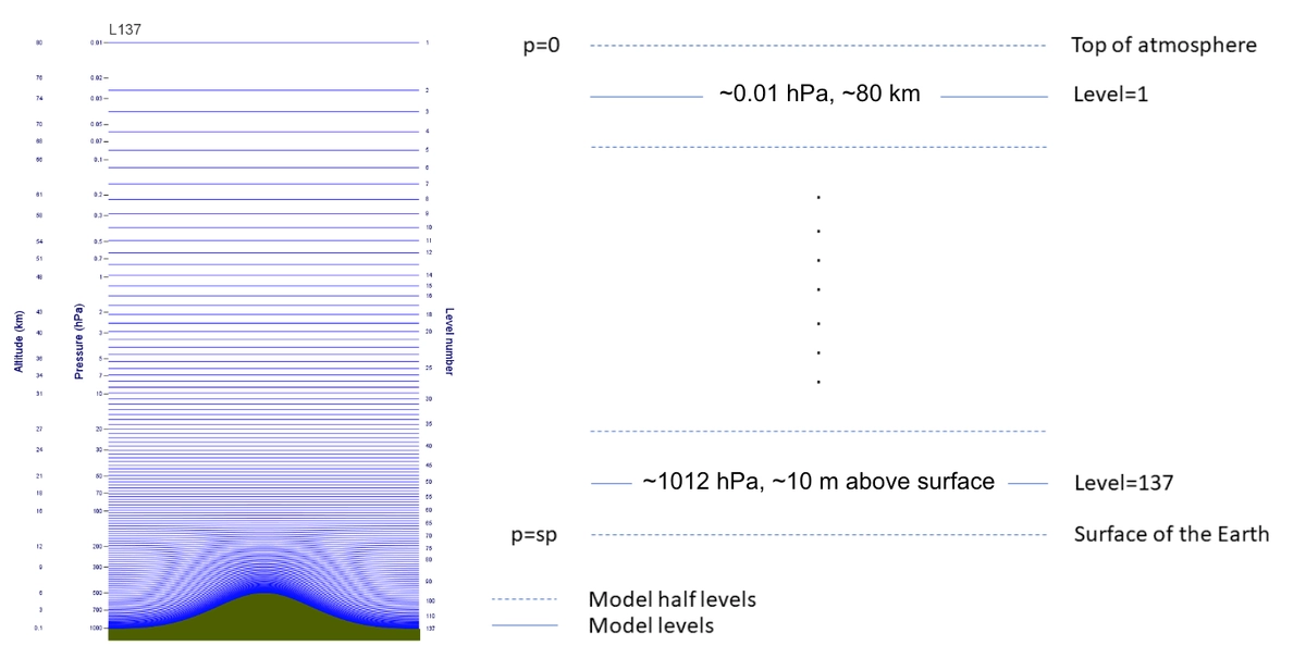
ECMWF IFS uses 137 model levels (MLs), numbered from top to bottom. ML1 is near 0.01 hPa (~80 km), while ML137 lies about 10 m above the model surface (~1012 hPa at standard surface pressure). Near the surface, the levels follow the terrain and are more closely spaced; ECMWF documentation
Another important aspect is time integration, which determines how the model advances from one time step to the next. Different numerical schemes can be used for this, depending on the model (for example, explicit, implicit or semi-implicit schemes).
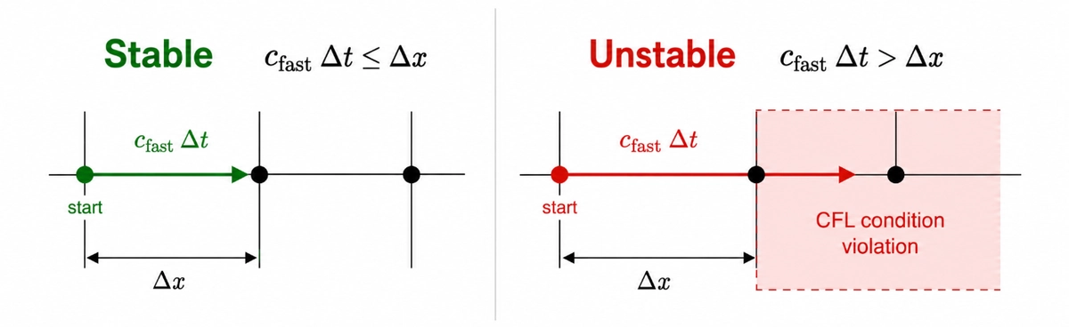
The length of the time step cannot, however, be chosen arbitrarily. For many numerical methods, it must be sufficiently short relative to the spatial resolution and the speed of the processes represented by the model. One of the fundamental stability criteria is described by the Courant–Friedrichs–Lewy (CFL) condition. In general, a finer grid therefore often means not only more grid points, but also a shorter time step and substantially greater computational cost.
Model physics and parameterisation
Model physics describes additional processes that influence atmospheric evolution but are not directly included in the dynamical core. These include, for example, radiation, cloud and precipitation formation, convection, turbulence, and processes occurring in the atmospheric boundary layer, at the Earth’s surface and in the soil.
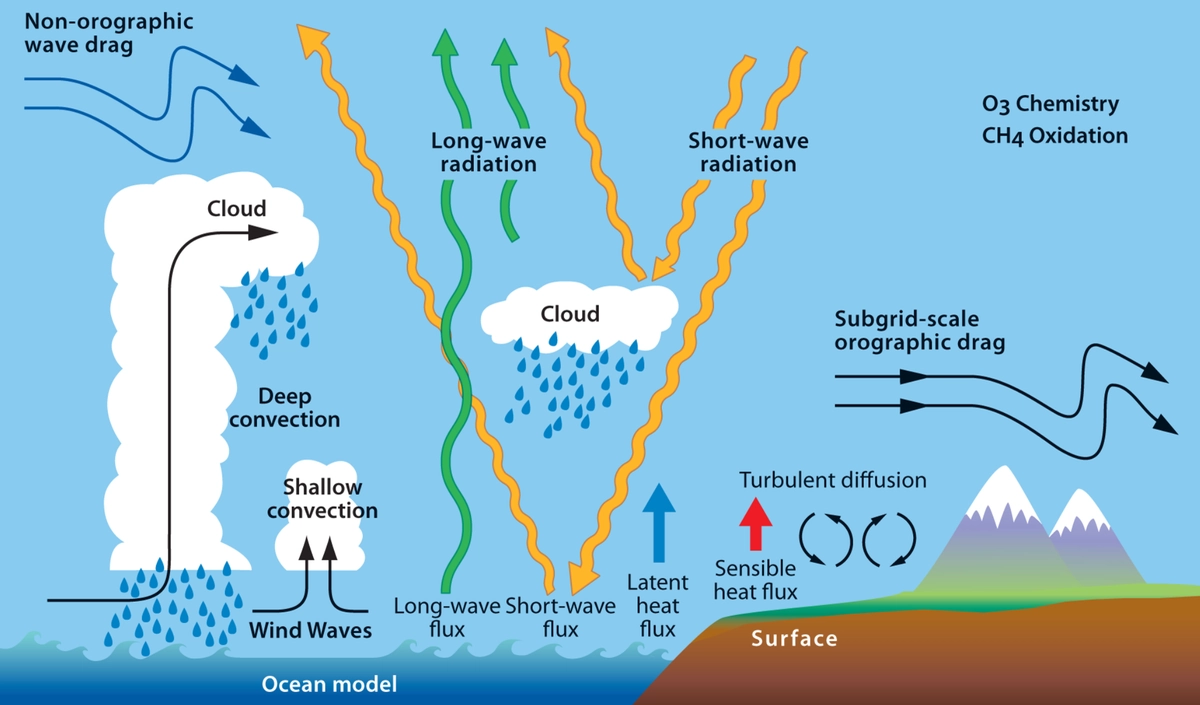
Schematic representation of processes included in the model physics; ECMWF
These physical processes are also closely interconnected and can create feedbacks, which the model should represent as realistically as possible. For example, changes in cloud cover affect radiation, which changes temperature and can in turn influence cloud formation.
Many of these processes occur on scales smaller than the model grid can resolve directly, or would be too computationally expensive to simulate in detail. Their effects are therefore often represented using parameterisations.
A parameterisation is a simplified mathematical representation of a physical process. It uses variables known to the model to estimate how that process affects the state of the atmosphere.
The principle of parameterisation can be illustrated well using cloud formation as an example. Within a single model grid cell, small saturated regions containing clouds may exist even when the average relative humidity of the entire cell is below 100%. The model therefore cannot simply assume that the whole cell is either cloud-free or fully saturated. A parameterisation estimates the amount of cloud, condensed water and precipitation, as well as their effects on temperature and moisture.
The choice of physical schemes in a model depends largely on its spatial resolution.
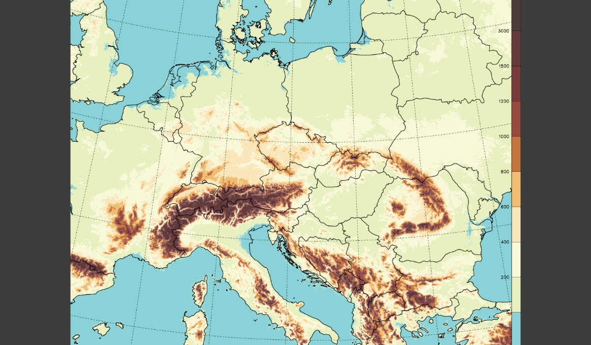
Orography of the ALADIN model operated by CHMI at 2.325 km resolution; CHMI
The model also requires additional information, such as orography, land-surface type, soil and vegetation, sea surface temperature, snow cover, sea ice and ozone concentrations. These data enter the calculation as auxiliary fields.
At each time step, the changes calculated by the dynamical core are combined with the effects of the processes represented by the model physics. In this way, the model advances the atmospheric state from one time step to the next.
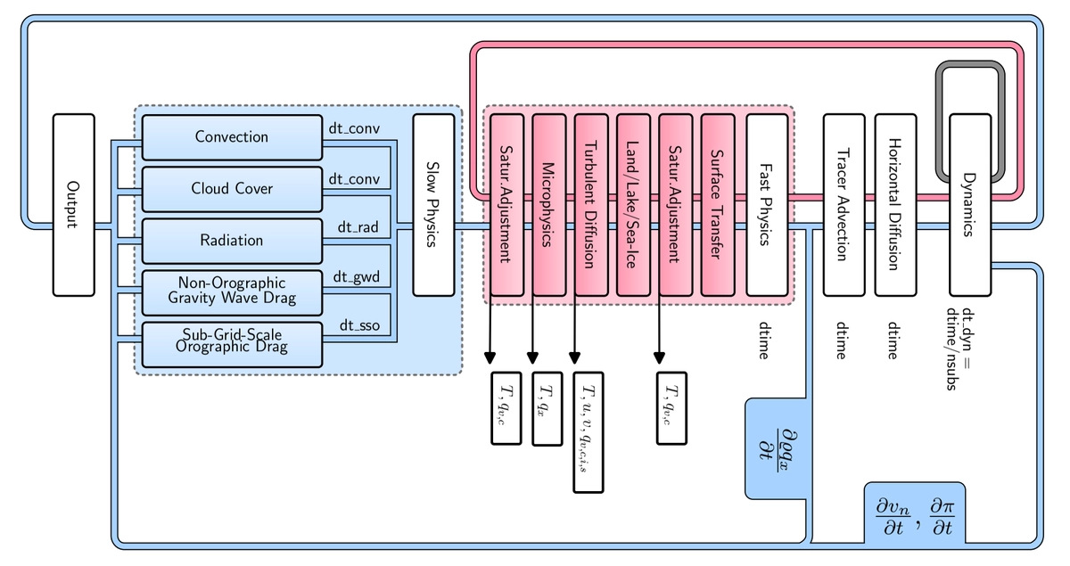
Coupling between the dynamical core and the NWP physics package in ICON; ICON Model Tutorial 2024
Domain and resolution: the whole world, or just part of it?
Every model has a defined domain, meaning the area for which it calculates a forecast.
Global models cover the entire Earth. This is particularly important for forecasts several days ahead, because weather at one location can later be influenced by weather systems thousands of kilometres away.
However, such a large domain comes with a high computational cost. Global models therefore generally cannot use grids as fine as those used by models covering smaller areas.

Example of a multi-grid setup with a global ICON domain at about 13 km resolution and a higher-resolution European child domain at about 6.5 km, similar to the operational ICON-EU setup; ICON Model Tutorial 2024
For more detailed forecasts, regional models with higher spatial resolution are used. Their finer grids allow them to represent features such as the influence of mountains, local airflow, and some aspects of intense convection in greater detail.
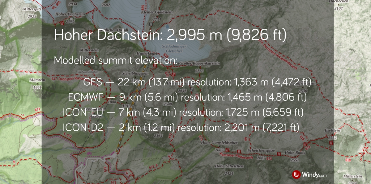
Regional models provide greater detail than global models, but their orography is still smoothed compared with reality, so forecast variables may not fully reflect local conditions
A regional model, however, also needs to know what is happening beyond the boundaries of its computational domain. It therefore usually receives this information from a global model or a larger regional model through lateral boundary conditions.
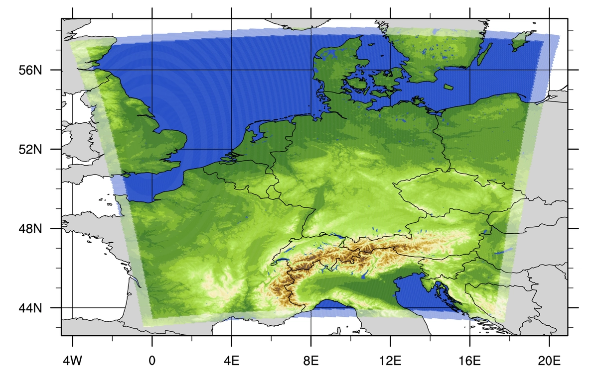
ICON-D2 model domain with a horizontal resolution of about 2 km. The highlighted 14-cell-wide lateral boundary zone consists of an interpolation zone (rows 1–4) and a nudging zone (rows 5–14), where the forecast is gradually adjusted towards the driving model; DWD
Initial conditions: the starting state of the atmosphere
We now have a numerical model based on the physical laws governing the evolution of the atmosphere, satisfying one of Bjerknes’s requirements. The next step is to determine its initial state as accurately as possible, thereby satisfying the other. The problem is that we do not have a sufficiently dense network of observations to cover every point on the model grid.
The first estimate is therefore usually taken from the previous model run, specifically its forecast valid at the initial time of the new run. In data assimilation, this is known as the first guess. This is then combined with current observations from many sources, including weather stations, radiosondes, radars, satellites, buoys, aircraft and wind profilers.
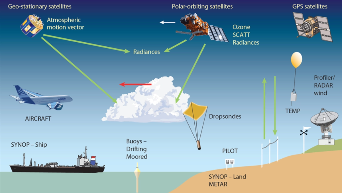
ECMWF receives around 800 million observations daily, with about 60 million quality-controlled observations available for use in the IFS. Most are satellite measurements, supplemented by surface and aircraft observations; ECMWF
However, observed values cannot simply be inserted at the nearest grid point to replace the original values. Doing so could disrupt the physical relationships between different variables.
Data assimilation is therefore used to combine the previous forecast with the observations. Its purpose is to create a state that matches the available observations as closely as possible while also respecting the physical structure of the model and the uncertainties associated with the different data sources.
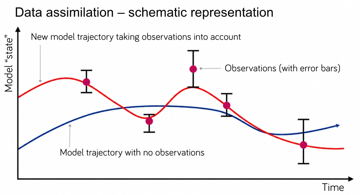
Data assimilation scheme: the impact of a new observation on the first guess (blue curve), leading to an analysis and an updated model trajectory (red curve); University of Reading
The result of data assimilation is an analysis, representing the best available estimate of the state of the atmosphere at the initial time. The new forecast run starts from this analysis.
Deterministic and ensemble forecasts
A single model run based on one analysis produces a deterministic forecast, representing one specific scenario of how the atmosphere may evolve.
However, the atmosphere is a chaotic system in which even very small differences in initial conditions can gradually lead to very different outcomes. At the same time, we can never know the initial state of the atmosphere with perfect accuracy. This sensitivity to initial conditions was famously demonstrated by Edward Lorenz in the 1960s.
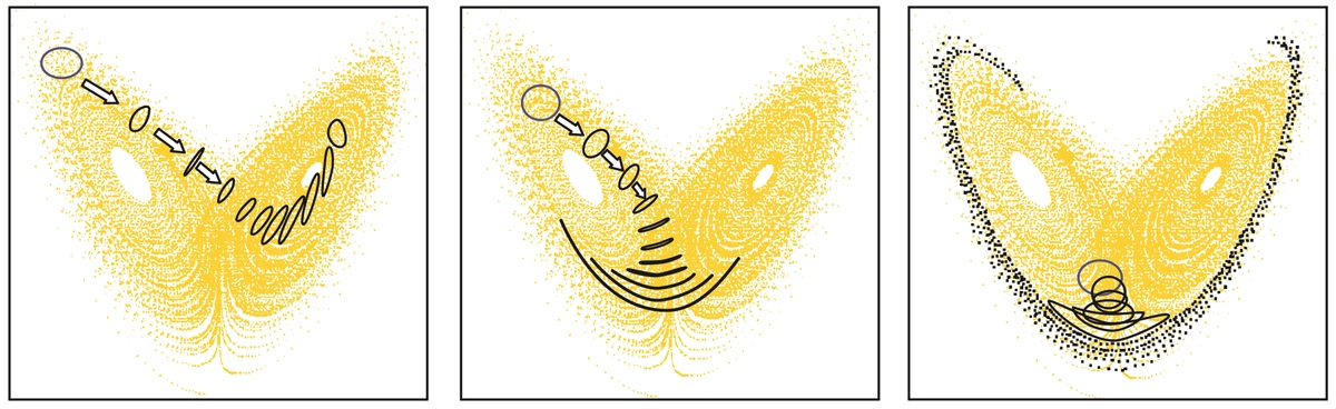
The Lorenz system illustrates the chaotic nature of the atmosphere: tiny differences in the initial state can lead to very different outcomes as the forecast progresses; T. N. Palmer
For this reason, ensemble forecasts are produced alongside deterministic forecasts. The model is run many times with slightly different initial conditions.
If the individual ensemble members evolve similarly, forecast uncertainty is lower. If they diverge significantly, uncertainty increases.
Ensemble forecasts therefore make it possible to work with the probabilities of different outcomes rather than a single scenario, and also to assess atmospheric predictability.
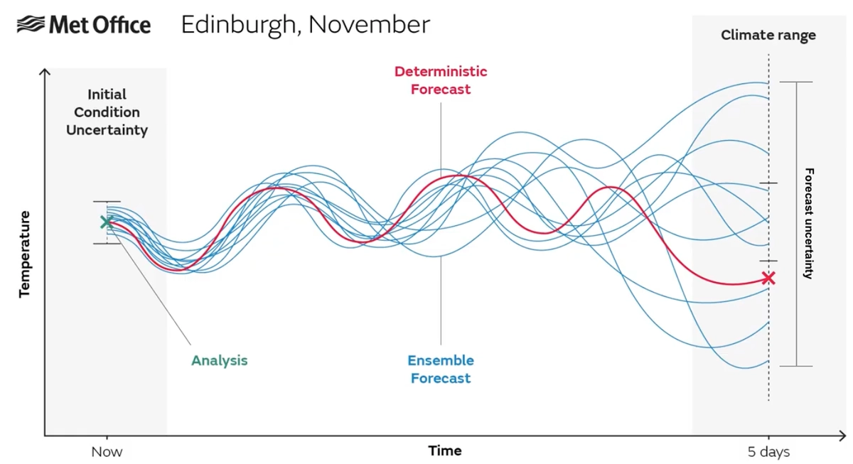
Each ensemble member is intended to represent an equally likely outcome, allowing the ensemble to be used to estimate the probability distribution of the predicted state of the atmosphere and to assess forecast uncertainty; Met Office via RMetS
You can read more about ensemble forecasts in the article Multimodel Approach to Weather Forecasting: Predictability and Probability.
The process does not end once the numerical calculation is complete.
Post-processing: from model output to a usable forecast
Raw model outputs are subsequently post-processed to make them better suited to practical use.
This may include, for example, converting data to common formats and time steps, interpolating to a specific location, correcting systematic errors, statistically calibrating, making local adjustments based on terrain, or combining multiple models.
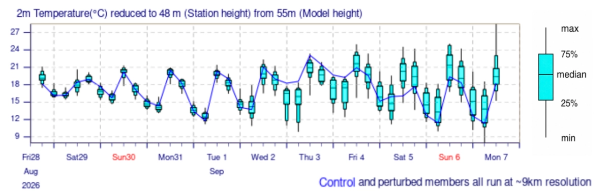
Post-processing may also include creating multimodel forecasts that combine information from multiple numerical models and leverage their distinct strengths. You can read more about this approach in the article Multimodel Approach to Weather Forecasting: Predictability and Probability.
At this point, we have the final forecast. However, its quality still needs to be verified.
Verification: evaluating forecast performance
Once the forecast period has been reached, it can be verified by comparing it with observations.
Verification assesses the magnitude of errors in forecast weather variables, as well as the forecast’s ability to capture extreme events. Various statistical verification metrics are used, such as bias (mean error), mean absolute error (MAE), root mean square error (RMSE), and different skill scores, which assess forecast quality relative to a reference forecast.
Verification helps identify weaknesses in the model and provides important information for its further development.
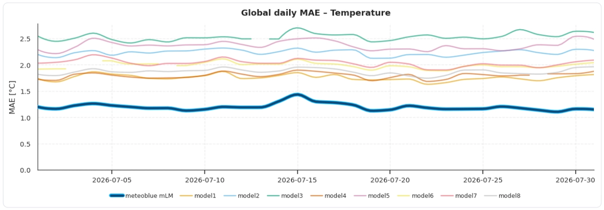
Daily global Mean Absolute Error (MAE) of the meteoblue Learning MultiModel and the global models IFS (ECMWF), AIFS (ECMWF), GFS, NEMSGLOBAL (NOAA/meteoblue), ICON, ARPEGE, UKMO and GEM for July 2026. MAE indicates how much the forecast differs from observations on average; meteoblue
When a new version of a model is being prepared, its results are tested on historical cases and compared with the previous version. The new configuration may then run in parallel with the current operational version for a period of time. Only if it demonstrates sufficient improvement can it be introduced into routine operations.
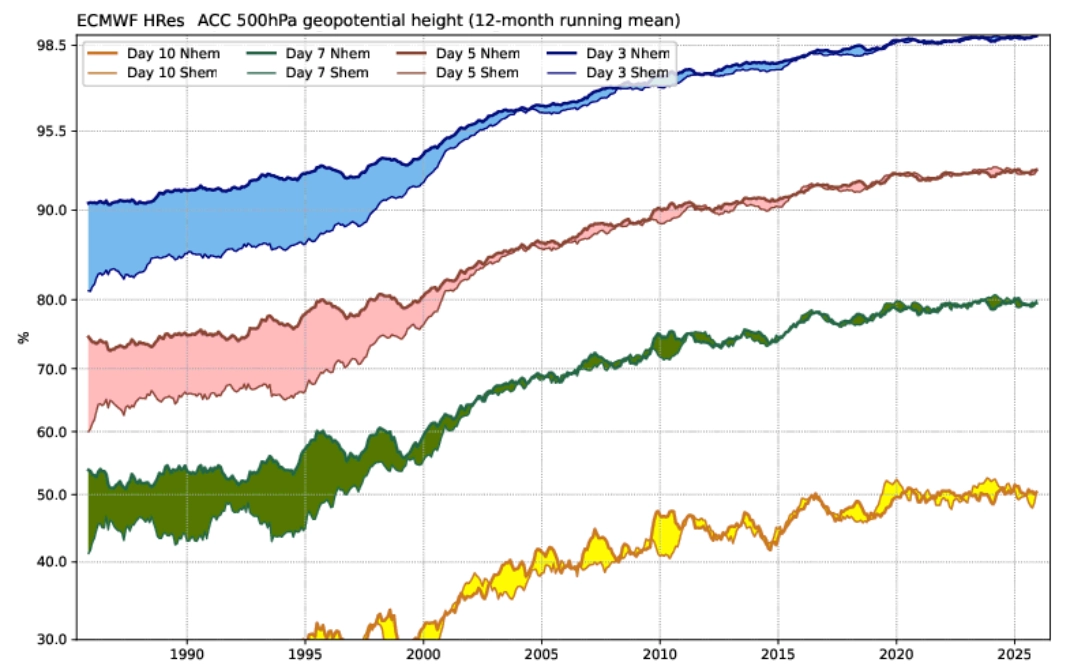
Evolution of ECMWF forecast performance for 500 hPa geopotential height in the Northern and Southern Hemispheres. The Anomaly Correlation Coefficient (ACC) measures how well the forecast reproduces the analysed large-scale atmospheric pattern; higher values indicate better forecast performance; ECMWF Charts
And then the whole cycle begins again: new observations arrive, a new analysis is produced, and a new forecast is generated from it.
Numerical weather prediction models on Windy.com
On Windy.com, you can view output from a wide range of global and regional numerical weather prediction models. ECMWF IFS, GFS and ICON are available worldwide, while selected regions also offer higher-resolution regional models such as AROME, ALADIN, HRRR, HRDPS, MSM, ACCESS and many others.
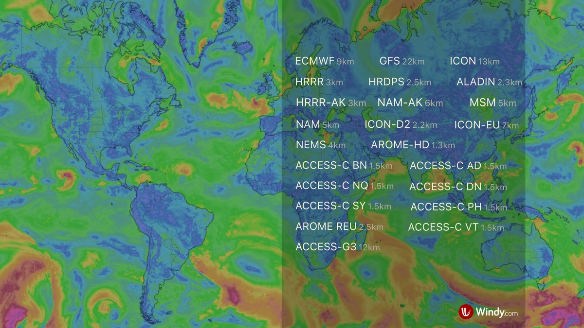
Numerical weather prediction models available on Windy.com
The individual models differ in their resolution, numerical methods, physical schemes, initial conditions and other components of the forecasting system. As a result, their forecasts may differ even when they start from the same reference time.
Basic information about each model, including which meteorological centre runs it, the initial time of the latest forecast run, the time of the most recent update and the expected time of the next update, can be found on Windy.com in the data information section.

meteoblue AI: The Most Accurate Global Forecast Model
Windy.com also offers the meteoblue AI multimodel point forecast. It is based on the meteoblue Learning MultiModel (mLM) system, which uses advanced post-processing methods, including statistical techniques and machine learning, to improve the output of numerical weather prediction models. Depending on the location, it combines output from approximately 30 to 40 models with current observations from weather stations, radars and other sources.
A 2025 verification study of the model across more than 30,000 stations worldwide found it improved precipitation forecast accuracy by over 20% compared to any single model, and it keeps getting better.
This is validated openly and on an ongoing basis. You can review the accuracy validation of the meteoblue mLM model in meteoblue's monthly verification reports, which continuously compare temperature, wind speed and dew point against other models.
Switch to your favourite model in the location forecast for more accurate weather.
meteoblue AI is available only as a location forecast for a specific place and cannot be projected onto a map. This is due to real-time recalculations that run in the background as data is gathered from all the weather models, weather radar, and the nearest weather stations for your location.
Comments (27)